
algorithms
research
Top-down mergesort with sorted check has mergecost (H+3)n
Simple proof that standard mergesort with a single extra comparison is run-adaptive in a rather strong sense.
We consider standard top-down recursive mergesort, where we do a single comparison before calling merge, to check whether the two recursively sorted subproblems happen to already be correctly ordered. (If so, we can skip the merging step.) We show that for any input $A[0..n)$ consisting of $r$ runs (maximal increasing contiguous subranges in $A$) of respective lengths $L_1,\ldots,L_r$, the mergecost $M$ (the sum of output sizes of all merges) satisfies $M \le (\mathcal{H}+3)n$ for $\mathcal{H} = \sum_{i=1}^r (L_i/n)\log_2(n/L_i)$ the runlength entropy.
Note that $\mathcal{H} n$ is a lower bound on the mergecost of any comparison-based sorting algorithm, so this shows that top-down mergesort with sorted check is run-adaptive in a rather strong sense. Moreover, the analysis is tight (in the sense that the constant 3 cannot be improved).
- A PDF version of this note is available on arXiv.
- Moreover, an interactive lab allows you to explore the recursion tree and charging scheme for any run-length profile, and to search for adversarial run-length profiles that push the mergecost to $(\mathcal{H}+3)n$.
Introduction
Run-adaptive sorting allows substantial speedups on partially sorted data, and is widely used in standard library implementations, e.g., in Timsort [Pet02] and Powersort [MW18]. A simple counting argument shows that the mergecost of any comparison-based sorting algorithm is at least $\mathcal{H}n$ in the worst case over all inputs with run lengths $L_1,\ldots,L_r$, and methods such as Peeksort [MW18], Powersort [MW18], and Length-Adaptive Shiversort [Jug24] guarantee a mergecost $M \le (\mathcal{H}+2)n$ (with the typical case being closer to the lower bound).
The above methods explicitly find the runs $R_1,\ldots,R_r$ in the input and then decide upon a clever order to merge them. In this note, we show the perhaps-folklore, but unpublished result that the following very simple algorithm achieves an only slightly weaker bound.
procedure Mergesort(A[l..r)):
    n := r - l
    if n <= 1 return
    m := l + floor(n/2)
    Mergesort(A[l..m))
    Mergesort(A[m..r))
    if A[m-1] > A[m]
        Merge(A[l..m), A[m..r), buf)
        copy buf to A[l..r)
We start by noting that $M$ can be written as
\[M \;=\; \sum_{i=1}^{r} M(R_i), \qquad M(R_i) \;=\; \sum_{\substack{v\in T:\\ R_i \subsetneq v \,\vee\, v \mathbin{⧉} R_i}} \lvert v\cap R_i\rvert, \tag{1}\]where $T$ is the recursion tree of standard mergesort, $v$ and $R_i$ are identified with their (integer) intervals of indices contained in their range, and the (nonstandard) notation $A \mathbin{⧉} B$ ($A$ “properly intersects” $B$) means that $A\cap B \ne \emptyset \wedge A \nsubseteq B \wedge A \nsupseteq B$, neither contained nor disjoint.
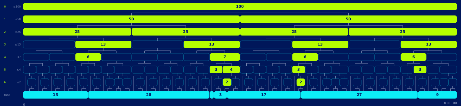
Figure 1: The recursion tree $T$ of mergesort on an input of size $n=100$ and run lengths $(L_1,\ldots,L_7) = (15,28,1,3,17,27,9)$. Nodes $v \in T$ that do not contain a run boundary are skipped (faded); only filled nodes contribute (their size) to the mergecost $M = 394$.
Equation (1) gives a charging scheme for the mergecost: each run pays for its contribution to the overall mergecost in the merges it participates in. Figure 2 gives an example.
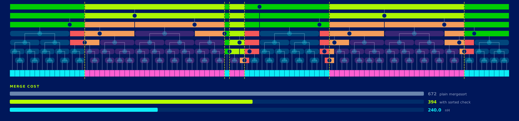
Figure 2: The recursion tree from Figure 1 showing the charging scheme of the analysis. Each run pays the colored parts in its vertical range.
A simple calculation shows that it suffices to prove that $M(R_i) \le L_i(\lg(n/L_i)+3)$, so in the following, we consider $M(R)$ for a single run of length $L$.
Power of two case
Without rounding, i.e., for $n$ a power of 2, the calculation is cleanest. We account for costs level by level. At depth $d$, a recursive subproblem has size $n/2^d$. We never need to charge $R$ more than $L = \lvert R\rvert$. At the same time, there can be at most 2 nodes $v\in T$ (recursive calls) at depth $d$ that contribute to $M(R)$ (cf. Figure 2), so charging $R$ at most $2\cdot n/2^d$ for depth $d$ also suffices, and we may take the minimum of the two. Hence1
\[M(R) \;\le\; \sum_{d\ge0} \min\lbrace L,\; 2\cdot n/2^d \rbrace \;\overset{(*)}{\le}\; L\cdot \lg\frac{n}{L} + 3L \tag{2}\]To see why inequality $(*)$ is true, set $G = \lfloor \lg(2n/L)\rfloor$ and $\theta = \lbrace \lg(2n/L)\rbrace = \lg(2n/L) - G \in [0,1)$. Then $2^\theta = 2n/(L2^G)$ and $2n/2^G = L2^\theta$. Now note that the minimum in the sum is $L$ iff $d \le G$; otherwise, for $d = G+k$, $k\ge1$, the minimum is $2n/2^d = (2n/2^G)\cdot 2^{-k} = L2^\theta\cdot 2^{-k}$. Thus
\[\begin{aligned} M(R) &\;\le\; (G+1)\cdot L \;+\; L\cdot 2^\theta \sum_{k\ge1} 2^{-k} \;=\; L\cdot\bigl(G+1+2^\theta\bigr) \\[.5ex] &\;=\; L\cdot\left(\lg\frac{n}{L} + g(\theta)\right) \qquad\text{with}\quad g(\theta) = 2-\theta+2^\theta \in [2.9,\,3]. \end{aligned}\]The last step uses $G = \lg(n/L) + 1 - \theta$. Note that $g$ is convex with $g(0) = 3$ and $g(\theta) \to 3$ as $\theta \to 1$, so it attains its maximum $3$ at the ends of the interval, and its minimum $2.9139\ldots$ at $\theta = \lg(1/\ln 2) \approx 0.5288$. The constant 3 is thus a trade-off, not slack: a large $\theta$ costs one level at the full charge of $L$, but fattens the geometric tail by the factor $2^\theta$, and the two effects cancel to within $0.09$ across the whole range.
General n
For general $n$, some recursive call sizes must be rounded up, so we have to make the analysis a little tighter. We need two new, but simple ingredients; the first relies on a ceiling fact.
Lemma 1 (Double Ceiling). For positive integers $n,p,q$, we have $\lceil \lceil n/p\rceil / q\rceil = \lceil n/(pq)\rceil$.
Proof. $\lceil n/m\rceil = \min\lbrace k \in \mathbb{Z} : km \ge n\rbrace$, and for integers $k$ and $n,p,q\in\mathbb{N}$ one has $kq \ge \lceil n/p\rceil \iff kq \ge n/p \iff kpq \ge n$. $\square$
The first new ingredient is a tight bound on the subproblem size for general $n$.
Lemma 2 (Node Sizes). Every node $v$ at depth $d$ satisfies $\lvert v\rvert \le \lceil n/2^d\rceil$.
Proof. Induction on $d$: the root ($d=0$) has size $n = \lceil n/2^0\rceil$. The child of a node of size $\le \lceil n/2^d\rceil$ has size at most $\lceil \lceil n/2^d\rceil/2\rceil = \lceil n/2^{d+1}\rceil$, using Lemma 1. $\square$
The second ingredient is that whenever $R \subsetneq v$ or $v \mathbin{⧉} R$ – that is, whenever $v$ contributes to $M(R)$ – the node $v$ must contain at least one element not in $R$, so
\[\lvert v \cap R\rvert \;\le\; \lvert v\rvert - 1 \;\le\; \lceil n/2^d\rceil - 1 \;\le\; n/2^d .\]We can thus still bound $M(R)$ by $\sum_{d\ge0}\min\lbrace L,\,2\cdot n/2^d\rbrace$ and obtain the bound (2) by the same calculation, which implies $M \le (\mathcal{H}+3)n$.
Note that the bound $M \le (\mathcal{H}+3)n$ is asymptotically tight: on input $(L_1,L_2,L_3) = (1,n-2,1)$, mergesort has $M = 3n - O(1)$, whereas $\mathcal{H} = O(\lg n/n)$.
Try it yourself
The interactive lab below draws the recursion tree and the charging scheme for any run-length
profile (click on charging colors for that). Drag the run boundaries in the strip at the bottom of the tree, or drag a run past its
neighbour to swap the two; the whole tree is rebuilt on every change. Switching on
charging colors and hovering a colored part shows the level-by-level breakdown of the bound
above for that run: the per-level charge against $\min\lbrace L, 2n/2^d\rbrace$, the closed form
$(G+1)L + 2n/2^G$, and the resulting $L\lg(n/L)+3L$.
The second tab runs an adversarial search over run-length profiles, so you can try to push $(M - \mathcal{H}n)/n$ past 3 yourself. (Hill-climbing reliably rediscovers the $(1, n-2, 1)$ family and stalls just below 3.)
References
[BW23] Gerth Stølting Brodal and Sebastian Wild. Funnelselect: Cache-oblivious multiple selection. European Symposium on Algorithms (ESA), pages 25:1–25:17, 2023.
[Jug24] Vincent Jugé. Adaptive Shivers sort: An alternative sorting algorithm. ACM Transactions on Algorithms, 20(4):1–55, August 2024.
[MW18] J. Ian Munro and Sebastian Wild. Nearly-optimal mergesorts: Fast, practical sorting methods that optimally adapt to existing runs. European Symposium on Algorithms (ESA), volume 112 of LIPIcs, pages 63:1–63:16, 2018.
[Pet02] Tim Peters. Timsort [listsort.txt], 2002.
-
The same calculation appears, e.g., in [BW23, §3.3]. ↩